Like a two-dimensional database, Excel is capable of storing many different types of data from small business contacts to personal income tax records. In both of these examples, accuracy is essential to make sure you have the information you need when you need it. In any data entry situation, people often transpose numbers or mistype a name in a spreadsheet. It is very difficult to tell the difference between 6886 and 6868 or 'John' and 'Johm' when you have long strings of numbers or text in a busy Excel worksheet.
Imagine when you do data analysis in Excel, one of the most frequent tasks is comparing data in each individual row. This task can be done by using the IF function, as demonstrated in the following examples. Using Excel's built-in function, you can make Excel do the work for you when you want to find out whether two cells contain exactly the same information. Continue to read to learn how you can automate the time-consuming task of checking for accuracy in your worksheets.
There are many ways to compare two columns. Let's go through the following steps to learn How to compare two columns in Excel.
Case Study 1: Compare two columns for matches or differences in the same row
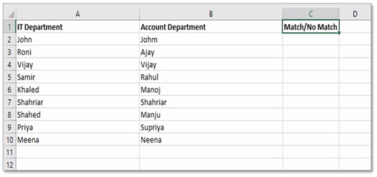
Step 1: Create a table same as like above picture. This table is showing the employee list of two departments. We will find the match of employee name between these IT and Account department. Column C will find the match between Column A and B in same row.
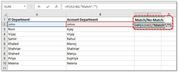
Step 2: In cell C2 we will use this formula:
=If(logical_test,"Value_if_True","Value_if_False")
In our case:
logical_test: A2=B2, Because we want to find match if the values of cell A2 and B2 are same
Value_if_True: Match, If found A2=B2 then the value of cell C2 will be "Match"
Value_if_False: "", If found "A2 is not equal to B2" then the value of cell C2 will be blank ("")
So, In cell C2 our formula will be:
=IF(A2=B2,"Match","")
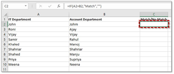
Step 3: Press ENTER. Now in cell C2 value is showing Blank (""), because there are no match between cell value of A2 (John) and Cell value B2 (Johm).
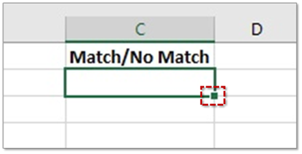
Step 4: Copy this formula from cell C2 down to other cells by dragging the fill handle (a small square in the bottom-right corner of the selected cell C2). As you do this, the cursor changes to the plus sign.
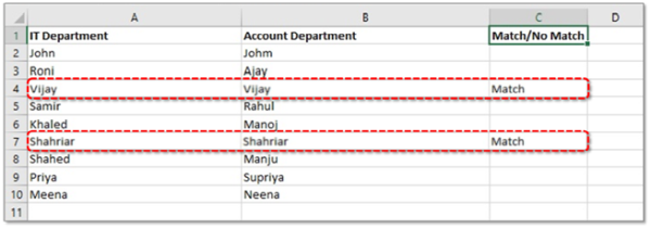
Step 5: After copy the formula to another cells of column C we will get the result of matching between two column A and B as like above picture. In the result we can see row 4 and row 7 has same employee name in both departments.
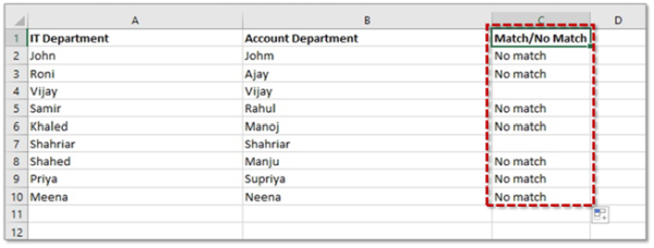
Tip 1: To find cells in the same row with different content, simply replace "=" with the non-equality sign:
=IF(A2<>B2,"No match","")
And do previous steps again. Then we will get result as shown in the image.
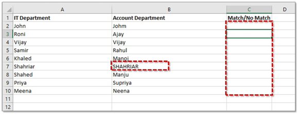
Case Study 2: Compare two lists for case-sensitive matches in the same row
Now we will find exact same name for case-sensitive matches.
Step 1: in Cell B7 Type ‘SHAHRIAR' instead of ‘Shahriar'. Delete all formulas from Column C.
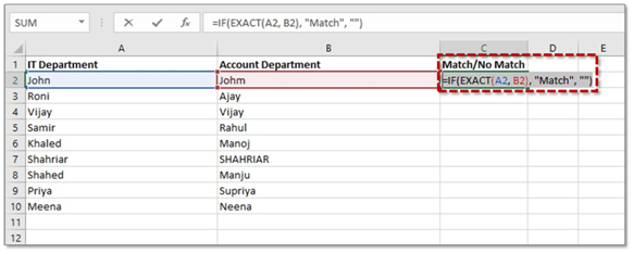
Step 2: Now use this formula in Cell C2:
=IF(EXACT(A2, B2), "Match", "")
Press ENTER and copy this formula to another cells of Column C.
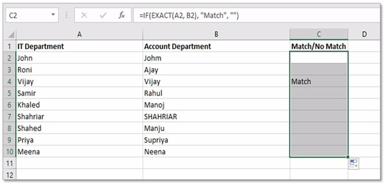
Step 3: Final result will be looked like above picture. Here we can see that after using case-sensitive match formula it found match only in row 4.
So, using IF function we can easily compare two or three columns based on our requirement, we just need to change the value of logical_test.
Now we have successfully learned how to compare two columns in Excel.
Recommended course to learn MS Office tools like Advanced Excel, Charts, PowerPoint Ninja, VBA Macros and Word for Finance Professionals.
Click here: /coaching/584-ms-office-bundle.asp


 CAclubindia
