Data cleaning is one of the necessary excel skills that you are expected to possess today. A data set might be having certain inconsistencies, and to make it more presentable and to help proper understanding of the data it is necessary to make the data look better and error-free.
Below, I mention 11 best techniques to help you 'clean' data.
Get Set Go.
#1. Run a Spell Check
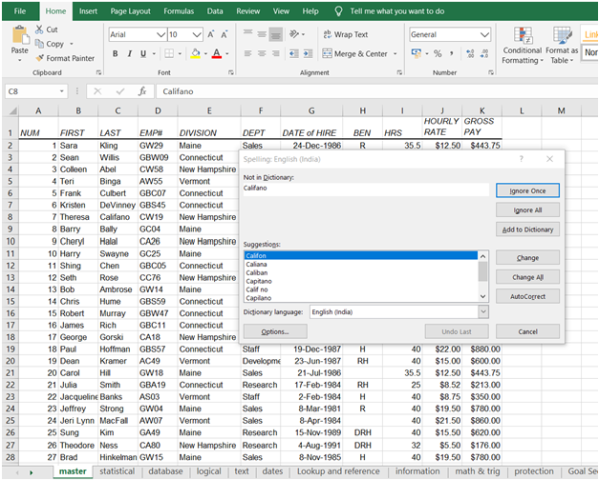
You'd agree that spelling errors are annoying. You wouldn't want anybody to question your dedication just because of some spelling mistakes or typos in your excel workbook. So, you must do a Spell Check before finalizing any excel document. You simply need to press keyboard shortcut F7 to open the Spell Check window and run the spell-check.

#2. Make the Text Case Consistent
You should make sure that the text case in the data is consistent. The data should not have some text in lower case, some in upper case and the remaining in proper case. To make the text case consistent throughout the data you can use the following functions, as required. Click on the function names below to learn how to use them.
UPPER - Converts text to Upper Case.
LOWER - Converts text to Lower Case.
PROPER - Converts text to Proper Case.
To learn more about click here
Extra spaces can make the data look clumsy. By extra spaces I mean more than one space between words and any spaces before of after the data string. Assuming you are working on a big amount of data, it can be next to impossible to spot and remove extra spaces manually. But you don't need to do this manually.
You can simply use the TRIM function to remove such extra spaces. You can click here to learn more about using the TRIM function.
#4. Clear All Formatting, Comments, Hyperlinks
You may have applied several kinds of formatting to the different parts of an excel file while working and while finalizing your work you might not be needing those formatting and may want to clear the data of all the formatting applied. Or you may have inserted several comments or hyperlinks for your references, which you now want to delete. You can clear all the formatting/comments / hyperlinks together for the whole data by simply selecting the data and going to Home --> Clear --> Select the appropriate option (Clear All / Clear Contents / Clear Comments / Clear Hyperlinks).
#5. Treat Cells Containing Errors
In a data, the cells containing errors can cause a lot of trouble for you when you sit down to analyze the data. So it is best to fix them. You can do this by either highlighting or selecting the cells containing errors.
Highlighting Errors
- Select the data.
- Go to Home --> Conditional Formatting --> New Rule. 'New Formatting Rule' dialogue box will open.
- Select ‘Format Only Cells that Contain’ option.
- In the Rule Description, select Errors from the drop down.
- Click on 'Format' button.
- Select the formatting options and click OK. This highlights all the errors in the data.
Selecting Errors
- Select the data.
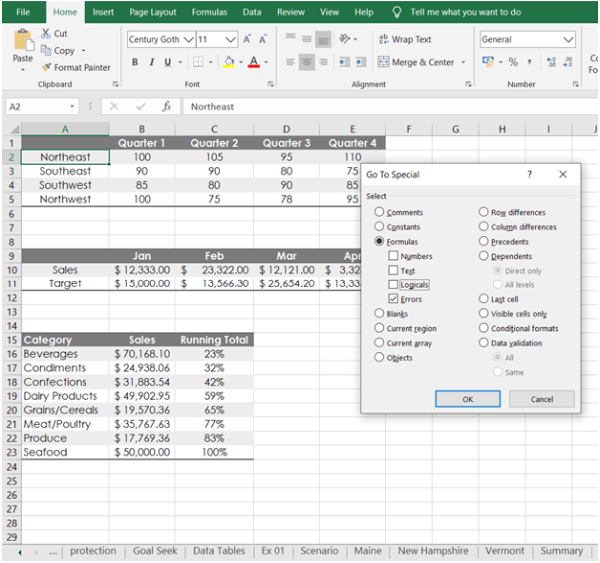
- Press F5 to open the Go To dialogue box.
- Click on 'Special...' button.
- Select Formulas and uncheck all the options other than 'Errors'.
- Click OK. All the cells containing errors.

#6. Use 'Find and Replace' Feature to Make Data Look Better
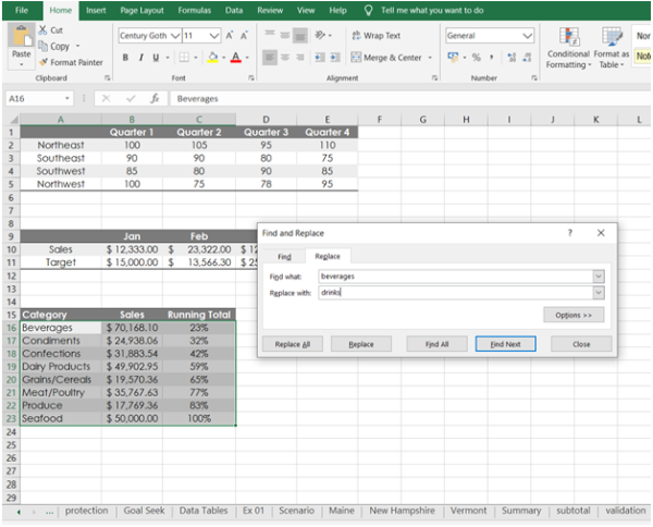
You can use the Find and Replace feature in Excel to replace certain ugly-looking text to their better-looking alternatives. For example, you can replace '&' (ampersand) with 'and'. You can replace error results viz. #N/A, #VALUE etc. with blanks or zeros as well (You first need to use 'Paste Special' to replace formulas with values.)
All you need to do is to select the appropriate cells and press keyboard shortcut Ctrl H. Then put the text you want to replace in the 'Find What' field, and the text you want to replace it with in the 'Replace With' field. Simple!

#7. Replace or Substitute Text
You can replace or substitute text in a column using formulas like REPLACE and SUBSTITUTE. You can use SUBSTITUTE when you want to replace specific text in a text string, and use REPLACE when you want to replace any text that occurs in a specific location in a text string. To know more about these functions, you can use the links given below:
#8. Replace Blank Cells with '0', 'No Value', Nothing', 'Not Available' etc.
Blank cells may cause many problems if you are converting the data into pivot tables or are making charts with the data. It is best to replace these blank cells with some appropriate data or text. It need a very simple exercise. Just follow the below steps:
- Select the data.
- Press F5 to open the Go To dialogue box.
- Click on 'Special…' button (or press Alt S). This will open the Go To Special dialogue box.
- Select 'Blank' option.
- Click OK. This will select all the blank cells in the selected data.
- Type the text ('Not Available', '0', etc.) and press Ctrl Enter. This will replace all the blank cells with the text.
#9. Treat Duplicates
The data maybe such that you don't want to have the same values more than once (or maybe you'd want to know which of the values appear more than once in the data).
To find duplicate values:
- Select the data.
- Go to Home --> Conditional Formatting --> Highlight Cells Rules --> Duplicate Values.
- Specify the formatting options and click OK. All the duplicate values in the data will be highlighted.
To delete duplicate values:
- Select the data.
- Go to Data --> Remove Duplicates.
- Select the Column(s) from which you want to remove duplicates and click OK. (If your data has headers, you need to check the checkbox 'My data has headers'.) All the duplicate data will be removed.
#10. Merging Contents of Columns
Sometimes you may need to merge the contents of two or more columns together to make the data more meaningful. You can easily do this by using & (ampersand) or the CONCATENATE function (not recommended). To know more about how to merge the contents of columns, please click here.
#11. Splittings Contents of a Column
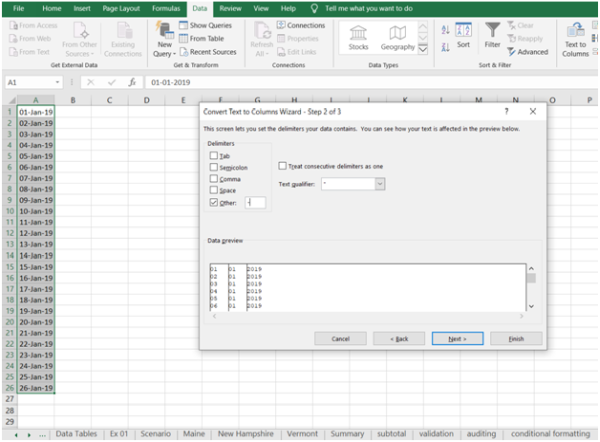
Contrary to the above, you may need to split the contents of the cells in a column. For example, you might need to split a column containing dates such that you have dates, months and years in separate columns. You can do this using the 'Text-to-Columns' feature in Excel. To know more about how you can use the Text-to-Columns feature, please click here.

Thanks for reading. See you soon. Happy Excelling!
(This article was originally published on my blog MadAboutExcel.com. To improve your knowledge in MS Excel, please visit my blog by clicking here.)


 CAclubindia
