Excel is a very important skill to have these days. There is a plethora of excel tips available on the internet. YouTube is full of Excel tips videos and channels. And there seems to be no end to how much we can learn in this spreadsheet software. There is virtually no limit to what we can do with and how much we can explore MS Excel. But still we use hardly a fraction of the functionalities Excel has to offer.
Below I give you a total of 14 important Excel tips that one is expected to know. This list of Excel tips is in no way exhaustive, but I am sure knowing these is a good starting point for anybody aspiring to gain deep knowledge in Excel.
So let's dive in!
1. Forget Mouse
To become truly efficient in Excel, you have to develop the habit of using a keyboard instead of a mouse. Using a mouse slows down the speed at which you work in Excel and can severely impact your efficiency. There are many keyboard shortcuts that you can use to save yourself a ton of time.
You can join my mailing list at madaboutexcel.com to get my course - "Ultimate Excel Shortcuts Course - Become 10X Faster on Excel" - for FREE. In this course, I'll show you how to use over 200 shortcuts to speed you up in Excel.
2. Leverage the Power of Paste Special
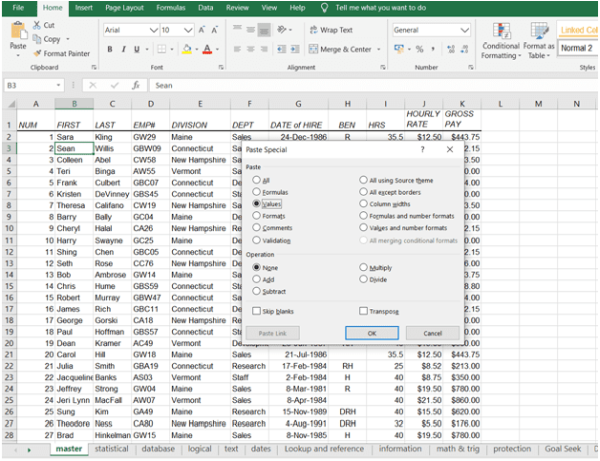
As I always say, Paste Special is a special feature in Excel. It has so many options and makes pasting data so much easier and this makes it is a must-know feature. You can even perform calculations and transpose data using Paste Special.
To open the Paste Special dialogue box, copy the data/cell and press the keyboard shortcut Ctrl Alt V after placing the cursor on the cell where you want to paste the data. Open the Paste Special dialogue box and explore all the options. I am sure you'll find them handy while working in Excel.
3. Use Comments to Keep Notes
Comments are a very useful, but highly underused feature of Excel. I use comments all the time to keep notes related to data in a cell or table so that I can refer to it later. I also use comments to note the details about a formula, so that I don't risk forgetting all about it when I look at the worksheet again after several days.
You can insert comments by right-clicking on a cell and Select Insert Comments option.
4. Use Freeze Panes
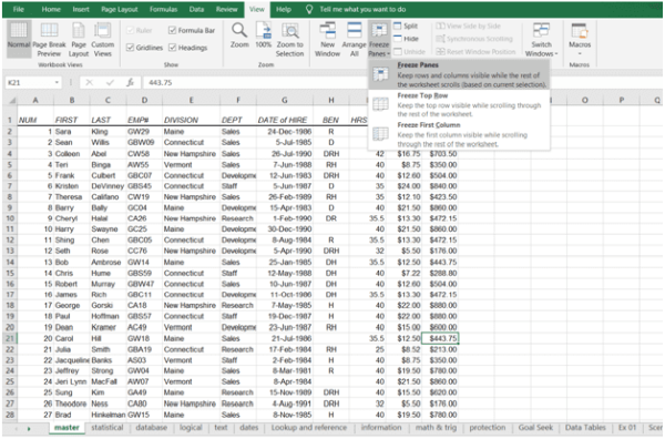
I hate scrolling up or left when working on a data having a large number or rows and columns. It is annoying to scroll up or left to see the row or column heads. So I use Freeze Panes option to lock the rows/columns so that the first row/column is always visible no matter how much I scroll down or right. The Freeze Panes option is available in the View menu.
5. Use Go To Special
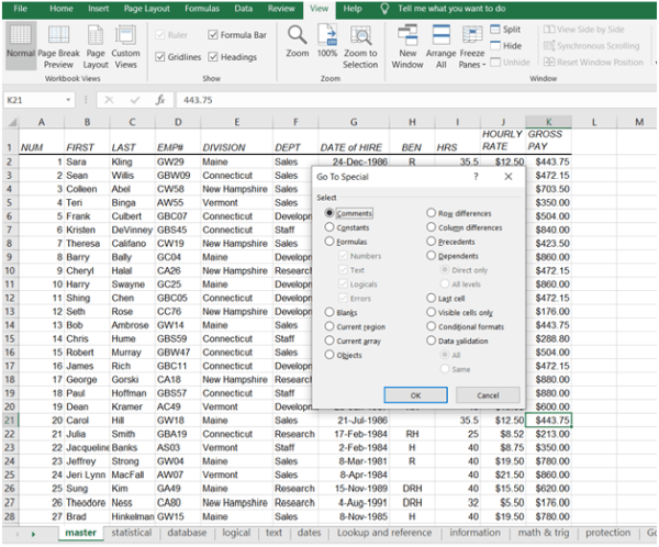
‘Go To Special' is again a very powerful feature in Excel. You can find and select various items in the entire worksheet with a single click using this feature. The items may be comments, formulas, blank cells, objects, precedents, dependents, conditional formatting, data validation etc.
I use this feature mostly when I need to find the cells with formulas, blank cells and objects.
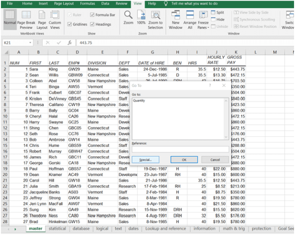
To access the Go To Special feature you just need to press Ctrl G to open the Go To dialogue box and then press Special button (or press keyboard shortcut Alt S). This will open the Go To Special dialogue box.
To learn more about the advance excel- CLICK HERE
6. Use Data Cleaning Techniques
In my previous post, I discussed the most important techniques to clean data in Excel. So, I won't get into a lot of detail in this post. Click here to read my post - "Ultimate Guide to Data Cleaning in Excel - 11 Super-Powerful Data Cleaning Techniques."
7. Protect Formulas
If you are working on documents that you'd be sharing with others, it is important to protect your work, especially the cells in which you have inserted formulas. Protecting formula cells is very important in the sense that any change in them can ruin all your hard work. That's why you should consider protecting the cells that contain formulas. The steps are given below:
Step 1: Select the entire sheet by pressing Ctrl A -> Press Ctrl 1 to open the Format Cells dialogue box -> Go to Protection tab -> Untick ‘Locked' and ‘Hidden' check-boxes -> Click OK
Step 2: Select a cell containing Formula -> Right-click on it and select Format cells -> Go to Protection tab and tick ‘Locked' and ‘Hidden' check-boxes -> Click OK
Step 3: Go to Review Tab in the Main Menu -> Click on Protect Sheet -> Provide a password (optional) -> Click OK
8. Format Painter
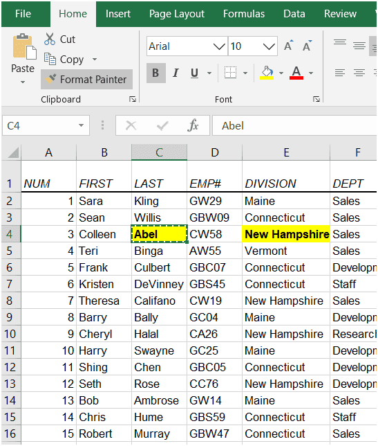
Format Painter is a very handy tool to quickly copy the formatting from one cell to other cell or cells. Clicking once on the Format Painter icon allows you to apply formatting to a single cell. If you want to apply the formatting to multiple cells, you'll need to double-click on the icon.
9. Explore More Sorting Options
Excel provides many sorting options. But most of us sort data in a column in either ascending or descending order and don't go beyond that. You might not know that you can sort data in excel based on values (ascending or descending), cell color, font color and cell icon.
Just click on filter drop-down and go to Sort by Color. There you'll see the Custom Sort option. Click on it to open the Sort dialogue box where you can explore these sorting options.
10. Differentiate Formula Cells with a Color Coding
Color coding different types of cells helps in organizing and analysis of data. One of the most common types of cells where color coding is applied to differentiate them from other cells, are the formula cells. By doing this, you know which values have been hard coded and which ones are the result of a formula.
To do this, press Ctrl G to open the Go To dialogue box. Click on the Special button. Select Formulas and click OK. Then, select the color highlight from the Fill Color button in the Home menu.
11. Leverage Named Ranges
The ability to assign a name to a range is another cool feature offered by Excel. Assigning a unique and descriptive name to a cell range give's the range an identity and helps you in recognizing it and referring to it in formulas. So instead of referring to a range as, say G1:J26 you can simply use the name of the range in the formula. This also saves time if you need to refer to a particular range several times.
You can access this feature by going to Formulas menu and clicking on Name Manager.
12. Tracing Precedents and Dependents
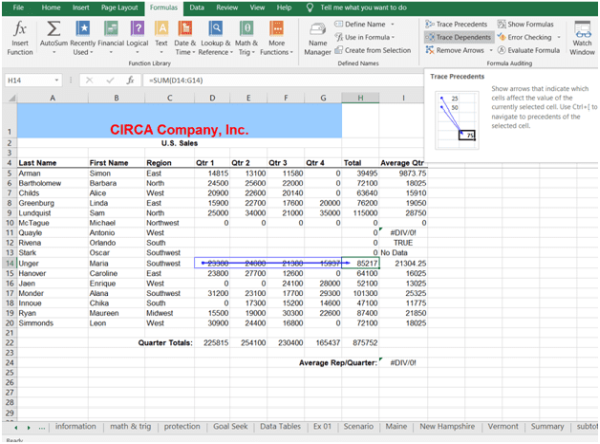
Sometimes, when working with big formulas and/or large data, it may become difficult to trace the cells on which the formula is dependent (precedents) or the cells which depend on the formula (dependents). You may need this information when you get lost in several formulas and are not sure which cells will be affected if you change some data.
It is very easy to know precedents and dependents of a formula. Select the cell containing the formula -> Go to Formulas menu -> Select Trace Precedent or Trace Dependent (as applicable) in the Formula Auditing group. Arrows will appear showing the cells dependent on the formula or the ones on which the formula depends (as applicable).
13. Avoid Hard-coding Formulas
Whenever I am writing a formula, I always make it point not to hard-code them.
Let me explain what I mean with the help of an example. Let's say I want to calculate interest on various amounts @ 8% which is the current rate of interest. Normally, one can write the formula as =A2*8%, A3*8% and so on. But what if the interest rate changes to 8.5%? You'll need to change the rate in all these formulas individually. So you should always write the interest rate in another cell and reference to it in the formulas. By following this method, you'll just need to change the value in the cell having the interest rate and all the changes will take effect automatically.
14. Managing Errors with IFERROR Function
Errors are common when it comes to using formulas in Excel. I find it really annoying to see errors like #N/A, #DIV/0!, #VALUE in my worksheets. To manage such errors, I use the IFERROR function. This function returns the value you specify if a formula evaluates to an error; otherwise, returns the result of the formula. To learn more about the IFERROR function, click here.
I am completely aware that I have not included a lot of similar tips above. But I never said that this is the end. I'll keep posting such lists in the future and continue giving you important tips to help you excel in Excel.
So what have I left out? What would you like me to include in the next list of Excel tips. I'd love to hear from you.
To learn more about the advance excel- CLICK HERE
The author can also be reached at vikram@madaboutexcel.com.
Thanks for reading. See you soon. Happy Excelling!


 CAclubindia
