Hey Friends!
Here is another tip related to financial analysis, which should be helpful to you guys.
Sorting from left to right
We all must have used sorting in lot of our exercises. We generally sort the data either alphabetically (A-Z or Z-A) or on the basis of values (increasing or decreasing) from “top to bottom”, but excel offers one more functionality which most of us are unaware of us, which is sorting data “left to right”. I will explain the trick here with its practical application in financial analysis.
How to do it?
As name suggests, here we will be sorting data from “left to right” in place of “top to bottom”. Let us try to appreciate its hands-on usage in our work through the exercise below.
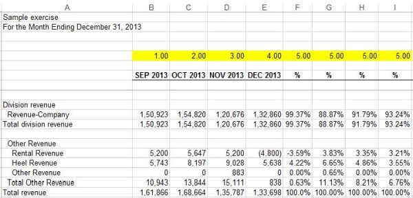
Consider the following set of data:
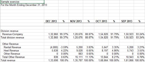
Now if we observe the data, we will notice the following 2 things:
- Data is available in reverse order (i.e. “December to September” in place of “September to December”)
- % are given in the data which is not relevant for us
This is the kind of output that we want:

One way of arranging/ cleaning the data for analysis, is to follow the following steps:
- Delete the unnecessary columns from data
- Then, manually re-placing the data in required order (using cut and paste function)
However, there is a systematic way of approaching towards the output shared above. Let’s discuss that:
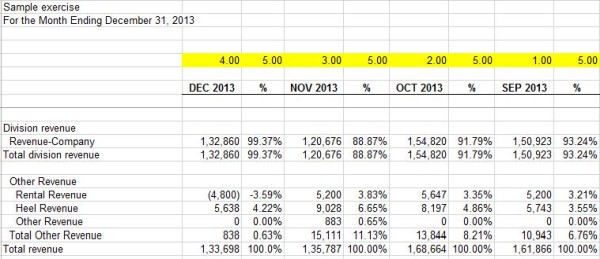
Step 1: We have to number the columns as shown in the image below. The numbering shall be in order that we want our output to be. Please note the following in the below image:
- Months- September to December have been assigned numbers 1 to 4 (on the basis of required output)
- All the irrelevant columns have been assigned last number which is 5 in our case so that after sorting, all these columns are shifted in the end
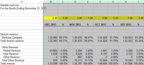
Step 2: Once the columns are numbered, follow the following steps
- Select the cells containing numbers
- Then, press “Ctrl + Enter” for selecting entire columns
By doing this, the entire columns shall be selected (Refer image below):
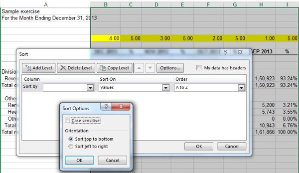
Step 3: In “Home” ribbon, there is an option for “Sort and filter”. Click there and then select “Custom sort”. A sorting window shall pop up with various options.
From there select “Options”. Another window shall open with 2 options viz “left to right” and “top to bottom”. By default it is top to bottom, but we have to select “left to right”. Refer image below:
Step 4: Once “left to right” is selected, enter the following details:
- Row no. on the basis of which data needs to be sorted (row no 5 in our case)
- On the basis of values
- Ascending or descending order
Once the above options are correctly selected, press OK and the desired output shall be obtained.
Remove the highlighted numbering. Hope this helps :) :)
Cheers!
Link to earlier articles:
- /articles/lets-excel-in-excel-funda-2-26876.asp (Funda 2)
- /articles/lets-excel-in-excel-funda-1-26828.asp (Funda 1)
P.S. A room without books is like a body without a soul - Marcus Tullius Cicer


 CAclubindia
