
In your day job, you have an excel workbook which is setup to get you the values you need, in the format you need. Probably using basic formulas, including VLookup.
Nothing is more annoying and depressing to get your carefully set VLookup formulas gets messed up. The bad part is, you might not know until it’s too late.
Consider this scenario, you have a table of GL code and GL balances. Somewhere else you are using a vlookup to find the closing balance of a GL.
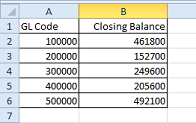
The Vlookup formula you use is following.
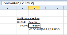
Check that you are looking up the second column. The Second column does not necessarily mean the balance of the GL. Imagine if somehow a column gets inserted between the balance column and the GL code column.
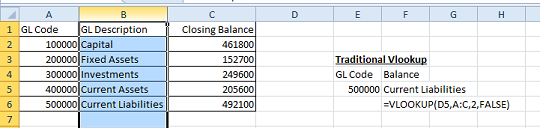
Now the same formula gives the GL description instead of the balance, which was intended & expected result from the formula. Since it is not throwing any error (#N/A, #Error, etc), there is a chance that you might not catch the change in time.
So, what is the solution?
Answer: the Formula "MATCH".
In simple language, Match function gets you the column number which matches the text you choose.
Below is a tweaked formula.
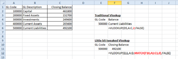
See the Red highlighted formula. There is no difference between the traditional VLookup and the tweaked one. We just replaced the "2" with MATCH formula.
In details of Match Formula:
=MATCH(F10,A1:C1,0)
The First field (F10) is the field which we want to search. This is the text "Closing Balance".
Second (A1:C1) refers to the table’s headers. Ie. GL Code, GL description and Closing Balance.
The last (0) refers to preference that we want to search exact text.
In summary, we want MATCH formula to find where the text is "Closing Balance" in the headers of the table. The answer to which is that it’s the 3rd column from right. This number we can use in our vlookup. Basically MATCH formula does what we manually do at the time of writing the formula.
Now the test, what would happen, if we insert a column in the table?
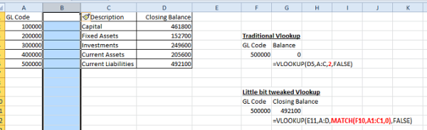
MATCH formula automatically updates the value to 4, and the VLookup results stay accurate.
Let’s delete few rows, and see if the results are still correct?
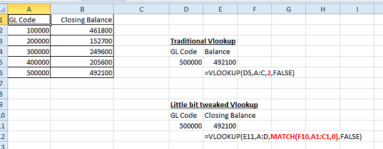
Now, what would happen, if I change the header of the column, of delete it altogether?
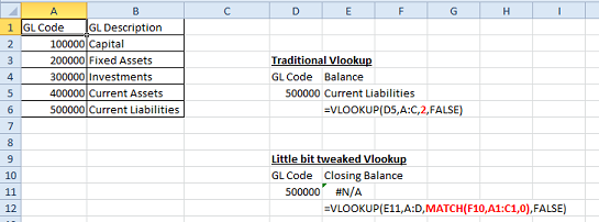
The formula gives #N/A, which will catch your attention. You can find where things went wrong.
Hope you find this article useful. If you have any queries, please write in the comments below, I will try to get back.











 CAclubindia