
Setup a pivot table
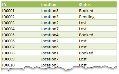
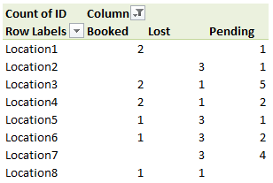
The first step is to just create a pivot table from this data. Put locations in row labels area, status in column labels are and ID in values area. Now you will have a count of items for each status in each location. Something like this:
Add a calculated item to get conversion ratio
Now we want to calculate how much percentage is “booked” status items in all items for a location. To do this,
- Select any column label item in the pivot table.
-
Click on Pivot Options > Fields, Items & Sets > Calculated item

- Give your calculated item a suitable name like Conv. %
-
Write the formula = Booked / (Booked + Pending + Lost)
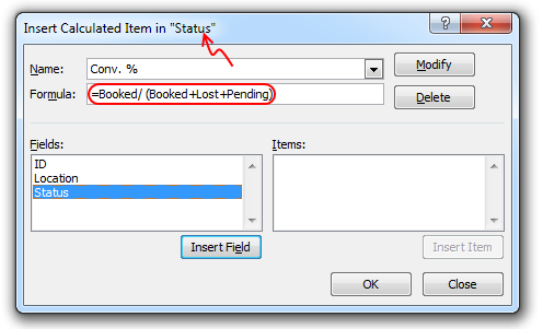
- Click ok.
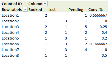
Now you should see another column in your pivot table with calculated item – Conversion %.
Formatting Conversion % in Percentage format
While we got what we wanted, it is not looking alright. We need to format the conversion % so that it looks alright. For this,
- Right click on any value in pivot table
-
 Go to value field settings
 - Click on number format
- Select custom
- Type the custom formatting rule [>=1]0;[<1]0%;”"
- This will automatically transform all numbers smaller than 1 (ie all conversion %s) to percentage format while keeping everything else normal.
- Done!
Attached File : 304961 1206232 conversion ratio.xlsx downloaded: 192 times


 CAclubindia
