
Understanding Vlookup.
The VLOOKUP function performs a vertical lookup by searching for a value in the left-most column of table_array and returning the value in the same row in the index_number position. Value is the value to search for in the first column of the table_array.
Syntax
VLOOKUP(lookup_value, table_array, col_index_num, match_type)
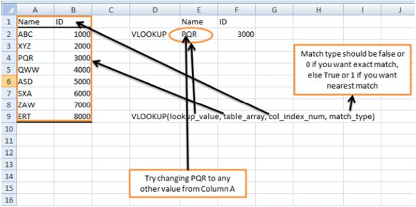
Cell F2 I have used vlookup function, and formula is: =VLOOKUP(E2, A2:B9,2,0)
Here lookup_value is value is the value to search for in the first column of the table_array, in our case it is value of cell E2,
table_array is two or more columns of data that is sorted in ascending order, in our case it is range A2:B9 ,
col_index_num is the column number in table_array from which the matching value must be returned. The first column is 1, for 2nd it is 2 & so on, in our case it is 2.
match_type is optional, It determines if you are looking for an exact match based on value. Enter FALSE to find an exact match. Enter TRUE to find an approximate match, which means that if an exact match if not found, then the VLOOKUP function will look for the next largest value that is less than value. If this parameter is omitted, the VLOOKUP function returns an approximate match.
If index_number is less than 1, the VLOOKUP function will return #VALUE!.
If index_number is greater than the number of columns in table_array, the VLOOKUP function will return #REF!.
If you specify FALSE for the not_exact_match parameter and no exact match is found, then the VLOOKUP function will return #N/A
(Refer attached sheet for explanation)
Attached File : 112266 1363166 vlookup.xls downloaded: 1235 times


 CAclubindia
