Excel data filter advanced command

To filter data: -

Video LInk - https://youtu.be/_TqxXqk_Jms

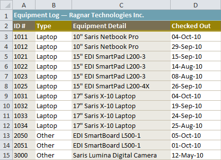
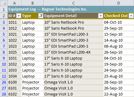
In this example, we'll filter the contents of an equipment log at a technology company. We'll display only the laptops and projectors that are available for checkout.

1. Begin with a worksheet that identifies each column using a header row.

   

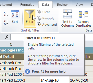
2. Select the Data tab, then locate the Sort & Filter group.
3. Click the Filter command.

   

4. Drop-down arrows will appear in the header of each column.
5. Click the drop-down arrow for the column you want to filter. In this example, we'll filter the Type column to view only certain types of equipment.

   

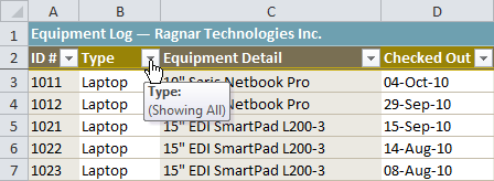
6. The Filter menu appears.
7. Uncheck the boxes next to the data you don't want to view, or uncheck the box next to Select All to quickly uncheck all.
8. Check the boxes next to the data you do want to view. In this example, we'll check Laptop and Projector to view only these types of equipment.

   

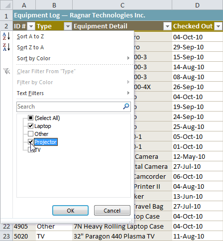
9. Click OK. All other data will be filtered, or temporarily hidden. Only laptops and projectors will be visible.

   

Filtering options can also be found on the Home tab, condensed into the Sort & Filter command.

Video LInk - https://youtu.be/_TqxXqk_Jms