" The Demand Curve "

Others 2186 views 12 replies

The Demand Curve


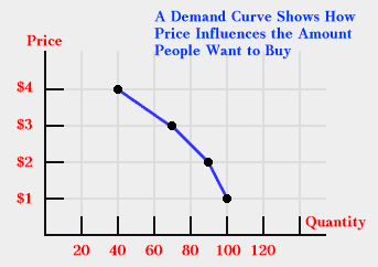
The relationship between price and the amount of a product people want to buy is what economists call the demand curve. This relationship is inverse or indirect because as price gets higher, people want less of a particular product. This inverse relationship is almost always found in studies of particular products, and its very widespread occurrence has given it a special name: the law of demand. The word "law" in this case does not refer to a bill that the government has passed but to an observed regularity.1


There are various ways to express the relationship between price and the quantity that people will buy. Mathematically, one can say that quantity demanded is a function of price, with other factors held constant, or:

Qd = f(Price, other factors held constant)


A more elementary way to capture the relationship is in the form of a table. The numbers in the table below are what one expects in a demand curve: as price goes up, the amount people are willing to buy decreases. (A widget is an imaginary product that some economist invented when he could not think of a real product to use in an example.)


A Demand Curve
Price of
Widgets
Number of Widgets
People Want to Buy
$1.00
100
$2.00
90
$3.00
70
$4.00
40

The same information can also be plotted on a graph, where it will look like

the graph below.2

Graph of Demand Curve
Replies (12)

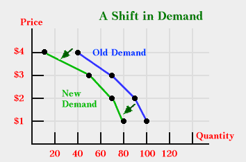
If one of the factors being held constant becomes unstuck, changes, and then is held constant again, the relationship between price and quantity will change. For example, suppose the price of getwids, a substitute for widgets, falls. Then, people who previously were buying widgets will reconsider their choices, and some may decide to switch to getwids. This would be true at all possible prices for widgets. These changes in the way people will behave at each price will change the demand curve to look like the table below.


A Demand Curve Can Shift
Price of
Widgets
Number of Widgets
People Want to Buy
$1.00
[100] becomes 80
$2.00
[90] becomes 70
$3.00
[70] becomes 50
$4.00
[40] becomes 10

These are the same changes shown in a graph.


A Shift in Demand 

Demand Terminology


If the price of widgets is originally $1.00 and people are buying 100, they may change to 90 for two reasons. One reason is that the price may rise to $2.00. The other reason is that one of the factors that is assumed to be constant may change, so that even though the price has not changed, quantity will. Economists distinguish these two cases. In the first case the demand relationship or schedule has not changed, but there has been movement within the relationship. Economists call a change of this sort a change in quantity demanded. The second sort of change is an alteration of the relationship. The original pairing of price and quantity is destroyed and replaced by a new pairing. Economists call this sort of change a change in demand.


It is important to realize that though the demand relationship looks concrete when it is illustrated with a table or graph, in everyday life demand curves are hidden. A demand curve refers to what people would do if various prices were charged, and very rarely are enough prices charged so a clear demand curve can be seen. This is not to say that the concept is of no importance to people who sell. They may not be interested in the demand curve as a relationship, but they do find it a boundary or constraint on their behavior. If there were an actual widget seller facing the demand curve in our demand table, he would find that he could not sell more than 90 widgets if he wanted to charge $2.00. He could of course sell fewer if he wanted to. He could sell only 70 at $2.00, but if he did this, he would earn far less than he could. If he wanted to sell more than 90, he would have to lower his price.


A Demand Curve
Price of
Widgets
Number of Widgets
People Want to Buy
$1.00
100
$2.00
90
$3.00
70
$4.00
40


Thus, to an actual businessman the demand curve is important as a limitation on what he can do. A businessman may not know exactly where the demand curve is, and he may not think of it as fixed. Advertising--either informing or persuading people--can move the boundary. As we proceed further, we will see that there are still other ways to view the demand curve in addition to seeing it as a mathematical relationship and as a boundary that limits sellers

Supply: Benefits and Costs


What determines the amount of a good or service that people are willing and ready to sell during some period of time? A discussion of exchange  suggested that people sell things because it is a way, indirect but effective, of obtaining other things that they prefer. Sellers intend to make a profit from their sales, and economists assume that they want their profits to be as large as possible. Because profit is the difference between benefits in the form of revenues and costs, anything that influences revenues or costs can influence the amounts sellers want to sell.


Revenue, the benefit that sellers get from producing and selling, is found by multiplying the price of the product by the amount sold. A change in price changes revenues and hence profits, so it is a major determinant of the amount sellers will want to sell. Because a higher price leads to higher profit, and a higher profit leads to a larger amount that sellers will want to sell, one expects that a greater quantity should be supplied when the price is higher. Thus, the relationship between quantity that sellers will sell and price should be direct or positive.


Though the positive relationship is almost always the case, there are a few exceptions. An example is labor; as wages go up, people may decide to enjoy their higher wages and work less. As a result, there is no law of supply that matches the law of demand.


The cost of something is what must be given up in order to get it. When costs are only monetary, they are easy to see. If the price of an input increases, the cost of the output will increase, and, other things held constant, profits will decrease. The seller will then have to decide if shifting part of his resources and effort to other products will improve his well-being.


Production costs are determined not only by the prices of inputs, but also by technology. Technology represents the knowledge of how inputs (such as labor, raw materials, energy, and machinery) can be combined to produce the product. If this knowledge increases so that people find cheaper ways to make the same output, then, other things held constant, profit increases and we expect sellers to respond by producing more.


Costs may be nonmonetary as well as monetary. For example, a farmer takes the expected price of soybeans into account in deciding how much corn to plant. If soybeans are expected to sell for a high price, then the farmer may find that shifting some of his land from corn production to soybean production will increase profit. The decision to plant corn means that the farmer gives up the opportunity to plant soybeans (as well as giving up the money for seed, fuel, equipment, and labor). Because we have defined cost as what must be given up to get something, the prices of other goods that sellers could otherwise produce and sell must be part of the calculation of the cost of production.


There are other factors that can influence the amount of a product that sellers will sell, such as the number of sellers, expectations about the future, and whether or not there are by-products in production that are valuable. (An example of a valuable by-product is cottonseed in the production of cotton. A farmer who produces cotton also gets cottonseed, which yields cottonseed oil, a widely used vegetable oil.) But as in the discussion of demand, the emphasis in the discussion of supply is on the relationship between quantity and price. To focus on  this relationship all other factors must be assumed to be constant.

The Supply Curve


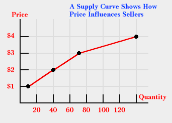
The relationship between the quantity sellers want to sell during some time period (quantity supplied) and price is what economists call the supply curve. Though usually the relationship is positive, so that when price increases so does quantity supplied, there are exceptions. Hence there is no law of supply that parallels the  law of demand


The supply curve can be expressed mathematically in functional form as


Qs = f(price, other factors held constant).


It can also be illustrated in the form of a table or a graph.


A Supply Curve
Price of
Widgets
Number of Widgets
Sellers Want to Sell
$1.00
10
$2.00
40
$3.00
70
$4.00
140

The graph shown below has a positive slope, which is the slope one normally expects from a supply curve.


The Supply Graph

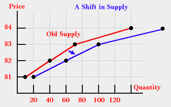
If one of the factors that is held constant changes, the relationship between price and quantity, (supply) will change. If the price of an input falls, for example, the supply relationship may change, as in the following table.

A Supply Curve Can Shift
Price of
Widgets
Number of Widgets
Sellers Want to Sell
$1.00
[10] becomes 20
$2.00
[40] becomes 60
$3.00
[70] becomes 100
$4.00
[140] becomes 180


The same changes can be shown with a graph that shows the supply curve shifting to the right. Notice each price has a larger quantity associated with it.


Supply Shift

Supply Terminology


As with demand, economists separate changes in the amount that sellers will sell into two categories. A change in supply refers to a change in behavior of sellers caused because a factor held constant has changed. As a result of a change in supply, there is a new relationship between price and quantity. At each price there will be a new quantity and at each quantity there will be a new price. A change in quantity supplied refers to a change in behavior of sellers caused because price has changed. In this case, the relationship between price and quantity remains unchanged, but a new pair in the list of all possible pairs of price and quantity has been realized.


Supply curves as well as demand curves appear much more concrete on an economist's graph than they appear in real markets. A supply curve is mostly potential--what will happen if certain prices are charged, most of which will never be charged. From the buyer's perspective, the supply curve has more meaning as a boundary than as a relationship. The supply curve says that only certain price-quantity pairs will be available to buyers--those lying to the left of the supply curve


The Model of Supply and Demand


To this point, we have developed two behavioral statements, or assertions, about how people will act. The first says that the amount buyers are willing and ready to buy depends on price and other factors that are assumed constant. The second says that the amount sellers are willing and ready to sell depends on price and other factors that are assumed constant. In mathematical terms our model is


Qd = f(price, constants)


Qs = g(price, constants)


This is not a complete model. Mathematically, the problem is that we have three variables (Qd, Qs, price) and only two equations, and this system will not have a solution. To complete the system, we add a simple equation containing the equilibrium condition:


Qd = Qs.


In words, equilibrium exists if the amount sellers are willing to sell is equal to the amount buyers are willing to buy.


If we combine the supply and demand tables in earlier sections, we get the table below. It should be obvious that the price of $3.00 is the equilibrium price and the quantity of 70 is the equilibrium quantity. At any other price, sellers would want to sell a different amount than buyers want to buy.


Supply and Demand Together at Last
Price of
Widgets
Number of Widgets
People Want to Buy
Number of Widgets
Sellers Want to Sell
$1.00
100
10
$2.00
90
40
$3.00
70
70
$4.00
40
140


The same information can be shown with a graph. On the graph, the equilibrium price and quantity are indicated by the intersection of the supply and demand curves.
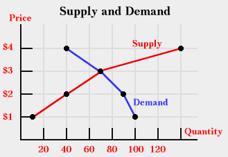
Graph of Supply and Demand Curves


If one of the many factors that is being held constant changes, then equilibrium price and quantity will change. Further, if we know which factor changes, we can often predict the direction of changes, though rarely the exact magnitude. For example, the market for wheat fits the requirements of the supply and demand model quite well. Suppose there is a drought in the main wheat-producing areas of the United States. How will we show this on a supply and demand graph? Should we move the demand curve, the supply curve, or both? What will happen to equilibrium price and quantity?


A dangerous way to answer these questions is to first try to decide what will happen to price and quantity and then decide what will happen to the supply and demand curves. This is a route to disaster. Rather, one must first decide how the curves will shift, and then from the shifts in the curves decide how price and quantity would change.


What should happen as the result of the drought? One begins by asking whether buyers would change the amount they purchased if price did not change and whether sellers would change the amount sold if price did not change. On reflection, one realizes that this event will change seller behavior at the given price, but is highly unlikely to change buyer behavior (unless one assumes that more than the drought occurs, such as a change in expectations caused by the drought). Further, at any price, the drought will reduce the amount sellers will sell. Thus, the supply curve will shift to the left and the demand curve will not change. There will be a change in supply and a change in quantity demanded. The new equilibrium will have a higher price and a lower quantity. These changes are shown below.
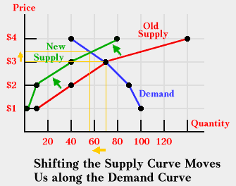
 

Shifting a Curve


What should one predict if a new diet calling for the consumption of two loaves of whole wheat bread sweeps through the U.S.? Again one must ask whether the behavior of buyers or sellers will change if price does not change. Reflection should tell you that it will be the behavior of buyers that will change. Buyers would want more wheat at each possible price. The demand curve shifts to the right, which results in higher equilibrium price and quantity. Sellers would also change their behavior, but only because price changed. Sellers would move along the supply curve.
 

Assumptions


The supply and demand model does not describe all markets--there is too much diversity in the ways buyers and sellers interact for one simple model to explain everything. When we use the supply and demand model to explain a market, we are implicitly making a number of assumptions about that market.


Supply and demand analysis assumes competitive markets. For a supply curve to exist, there must be a large number of sellers in the market; and for a demand curve to exist, there must be many buyers. In both cases there must be enough so that no one believes that what he does will influence price. In terms that were first introduced into economics in the 1950s and that have become quite popular, everyone must be a price taker and no one can be a price searcher. If there is only one seller, that seller can search along the demand curve to find the most profitable price.1 A price taker cannot influence the price, but must take or leave it. The ordinary consumer knows the role of price taker well. When he goes to the store, he can buy one or twenty gallons of milk with no effect on price. The assumption that both buyers and sellers are price takers is a crucial assumption, and often it is not true with regard to sellers. If it is not true with regard to sellers, a supply curve will not exist because the amount a seller will want to sell will depend not on price but on marginal revenew


The model of supply and demand also requires that buyers and sellers be clearly defined groups. Notice that in the list of factors that affected buyers and sellers, the only common factor was price. Few people who buy hamburger know or care about the price of cattle feed or the details of cattle breeding. Cattle raisers do not care what the income of the buyers is or what the prices of related goods are unless they affect the price of cattle. Thus, when one factor changes, it affects only one curve, not both. When buyers and sellers cannot be clearly distinguished, as on the New York Stock Exchange, where the people who are buyers one minute may be sellers the next, one cannot talk about distinct and separate supply and demand curves.


The model of supply and demand also assumes that both buyers and sellers have good information about the product's qualities and availability. If information is not good, the same product may sell for a variety of prices. Often, however, what seems to be the same product at different prices can be considered a variety of products. A pound of hamburger for which one has to wait 15 minutes in a check-out line can be considered a different product from identical meat that one can buy without waiting.


Finally, for some uses the supply and demand model needs well-defined private-property rights. Elsewher, we discussed how private-property rights and markets provide one way of coordinating decisions. When property rights are not clearly defined, the seller may be able to ignore some of the costs of production, which will then be imposed on others. Alternatively, buyers may not get all the benefits from purchasing a product; others may get some of the benefit without the payment


Even if the assumptions underlying supply and demand are not met exactly, and they rarely are, the model often provides a fairly good approximation of a situation, good enough so that predictions based on the model are in the right direction. This ability of the model to predict even when some assumptions are not quite satisfied is one reason economists like the model so much

Buyer and Seller Equilibrium


We have developed the model of supply and demand as an equilibrium model. We have said nothing about how adjustments from disequilibrium to equilibrium take place. To develop this idea, it is useful to take still another view of supply and demand curves, to view demand as points of buyer equilibrium and supply as points of seller equilibrium.


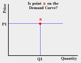
Is this point on the demand curve?


Suppose that price is at P1 in the graph above. Will point a be a point on the demand curve? If people would like to buy more than Q1 at price P1, point a must lie to the left of the demand curve. In this case, some consumers are unhappy with the amount they have purchased and will try to purchase more. If there is no more to purchase, some will attempt to offer more money for the product or they will increase the time they devote to getting the product. The important idea is that if point a lies to the left of the demand curve, people will be unhappy with their situation and will change their behavior. If point a lies to the right of the demand curve, people will decide that they are buying too much of the product and will cut purchases. In conclusion, if a position is not on the demand curve, people will change their behavior, which indicates that only positions on the demand curve are positions of buyer equilibrium.


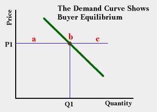
Similar reasoning explains why the demand curve can be considered a boundary. In the graph below, buyers are not in equilibrium at point a, but they can be held there and made to adjust in ways that do not change the money price. They cannot be held at point c unless there is some way to force people to buy a product when they do not want it.

Demand Curve shows buyer equilibrium


Point b in the graph is a position of buyer equilibrium because, given price P1, people will be satisfied with Q1 and will do nothing to change their behavior. Buyers would, of course, prefer a lower price than P1--they are always willing to move down the demand curve. However, this is not the issue here. Given P1, Q1 is the preferred quantity.


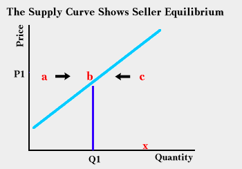
Just as the demand curve shows positions of buyer equilibrium, the supply curve shows positions of seller equilibrium. At point a in the picture below, suppliers find that they could increase profits (or reduce losses) by moving to the right to a larger quantity. If they could not increase profits by moving toward the right, they would stay at point a. Because they do not, they are not in equilibrium and on the supply curve but to the left of it. If they find that they could increase profits by cutting production, they are to the right of the supply curve and out of equilibrium. There is a quantity at the price P1 that maximizes profits and toward which sellers will adjust. This point, shown as b in the picture, is on the supply curve.


Supply curve shows seller equilibrium


It is possible to force sellers to a position left of the supply curve. This is the case in which sellers would like to sell more at the given price, but for some reason can not. One reason might be that the buyers will not buy as much as the sellers would like to sell. It is virtually impossible--short of slavery--to force sellers to the right of the supply curve. If sellers are selling more than they want to at the given price, they can simply stop selling. Thus, the supply curve represents a boundary facing the buyers. If buyers could force sellers to the right of the supply curve, they would find it advantageous to force sellers to a position such as x in graph above, which represents getting something for nothing.


Sellers prefer higher prices to lower prices. Although all points on the supply curve represent points of equilibrium, not all are equally preferred by sellers. Sellers are always happy to move up along a supply curve.

Shortages and Surpluses


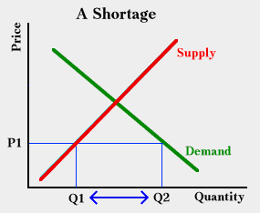
Viewing points on the demand curve as points of buyer equilibrium and points on the supply curve as points of seller equilibrium helps explain how an adjustment process takes place in the supply and demand model. If price is originally P1 in the graph below, only Q1 will be sold even though buyers would like to buy Q2. The difference Q2 - Q1 represents a shortage. The sellers are in equilibrium in this situation because they can sell everything they want to sell at this price, but buyers are not. Some buyers who cannot obtain the product are willing to offer more, and sellers are always willing to accept a higher price. Therefore, the actions of the buyers, as they compete with each other to obtain the amount that is available, drive the price upward in this model toward market equilibrium.


A Shortage


If price is originally at P1 in the picture below, only Q1 will be sold because this is all that buyers will purchase, even though sellers are willing to sell more, Q2. The difference Q2 - Q1 is called a surplus. In this situation the buyers are in equilibrium because they can buy all they want to buy at the going price. However, the sellers are not in equilibrium and will compete among themselves to get rid of the surplus. Some sellers will be willing to offer their product at a lower price. Buyers are always willing to move down the demand curve, so there is a tendency to move downward toward market equilibrium in the picture below.

A Surplus

If left to itself, a supply-and-demand market tends to adjust to the point where the supply and demand curves cross. The price at this intersection is called the market-clearing price. There is, however, the possibility that the existence of lags in the adjustment process may make the adjustment more complex than the previous discussion indicates.


Suppose that the price of cattle feed rises sharply. This event should affect the supply curve of cattle by shifting it to the left. The profitability of cattle production is reduced at each possible price, and some producers will drop out of the industry while others will curtail production. Looking at the curves, we see that price should rise and quantity should drop. However, initially price might drop and quantity might rise, which is the exact opposite of the prediction from the supply and demand graph. The higher costs of feed will encourage farmers to raise fewer cattle, but as part of that cutback, they will temporarily send more cattle to the slaughterhouses. The prediction that supply-demand analysis gives will ultimately be correct, but it will not be correct in the process of adjustment.


More complicated adjustment patterns are possible. Suppose, for example, that higher beef prices shift the demand for pork to the right. Supply and demand analysis says that this should increase pork prices, and at the higher prices, farmers should produce more hogs.


However, hog production takes time, and will only happen if farmers expect the higher prices to continue for a long time. If pork producers do expect the higher prices to last, they may decrease the number of pigs sent to slaughter, further increasing price. A sow can either produce pork or baby pigs, but not both. If farmers expect high prices to last, they will keep their sows for piglet production.


In six months to a year, the baby pigs will have grown enough to go to market. If enough farmers had expected the high prices to last, they may have produced so many pigs that pork prices will now plunge to a level below that which is considered normal. The new, abnormally low price can then influence decisions that will not affect the price for many months. You should see that, once disturbed, a market with long time lags in production may bounce around for years before it finally finds its way back to equilibrium. If such a market is disturbed often enough, its prices and quantities will never come to rest at equilibrium levels.


Microeconomic discussion generally ignores adjustment problems, at least at the introductory level. Microeconomics assumes that markets clear, that is, they are always in equilibrium. Its analysis begins with the assumption that equilibrium has been reached and then asks questions about that equilibrium. However, adjustment problems are very important in macroeconimics. Macroeconomics cannot assume there are no adjustment problems or else it assumes away one of the problems it wants to explain, unemployment. In fact, much of macroeconomics is about the forces that bump an economy away from equilibrium, and why, once it is away, it has problems reaching a new equilibrium.

thnx 4 sharing

 Thanx yar..........tumne to puri chapter hi upload kardi...................

thanx 4 sharing


CCI Pro

Leave a Reply

Your are not logged in . Please login to post replies

Click here to Login / Register