
Lookups in Microsoft Excel, most of us always preferred to go with VLOOKUP as it is regarded as a basic lookup function in Microsoft Excel and also essential for those who willing to work or already worked on Excel to have detailed understanding of this productive function.
But most of us are aware that this function can be useful to extract only first row information yes it correct in someway as Microsoft is also certified it. They mentioned that “You can use the VLOOKUP function to search the first column of a range (range: Two or more cells on a sheet. The cells in a range can be adjacent or nonadjacent.) of cells, and then return a value from any cell on the same row of the range”
But in my view it is partially correct. We can extract multiple row Information by using Vlookup function also.
Now let see how we extract multiple row information by using Vlookup Function.
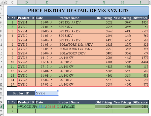
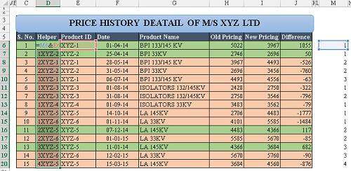
Suppose we have price history of M/s XYZ for the year 2015 and our goal is to extract date wise and product wise price changes information.

Now by using simply Vlookup function we get only first row information.
But if we follow this trick we can extract multiple row information. The details steps are under
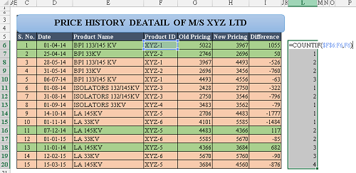
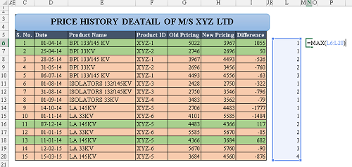
Step 1: Create sequential number for each changes for each product by writing this formula =COUNTIF($F$6:F6,F6) on anywhere on excel sheet and copy the same paste it for same number of sequence and also enter max function for getting aware what is the maximum number of changes for any product.
Step 2: Create A new column before Product ID column
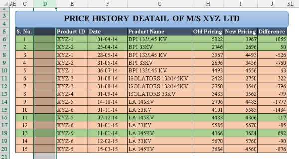
Step 3: Create this formula on “D6” =O6&F6 and paste on entire range i.e. on D6 to D20. This will gives a unique identification keys, even for same product which are changed.
Step 4: Put sequence under S. No by referring to maximum number referred to step 1

Step 5: Now select a range D25:J28 and put a modified Vlookup function =VLOOKUP($C25&$F$22,$D$6:$J$20,COLUMN(A1),FALSE) on D25 and hit enter by pressing Ctr key.
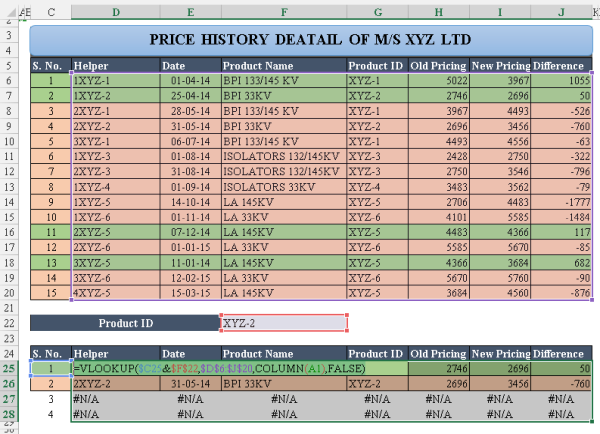
Instantly you will get all price revision for each product. (Column (A1) will give 1 and Column (B1) gives 2 and so on)
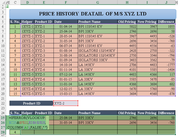
Further there might be #N/A types of errors for those case in which No of price changes are less than 4. In that case you need to add one more function in step 5 it is iferror function in the following way =IFERROR(VLOOKUP($C25&$F$22,$D$6:$J$20,COLUMN(A1),FALSE)," ") it works on the principle that if error is there by Vlookup function it simply gives blank (in Microsoft Excel blanks are represented by “ “)
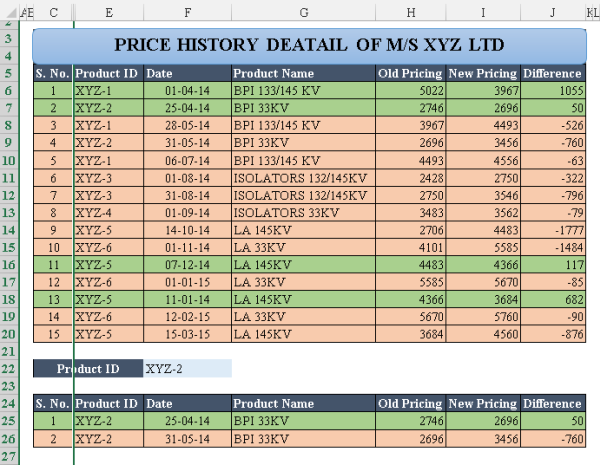
Step: 6 Hides all non-relevant columns for reporting purposes
Note: 1. in this workbook some Advance Conditional Formatting function is also operating, and how it works will be mentioned in future articles
Note: 2. In S. No. also have some advance and conditional function for dynamic references, however it is difficult to explain the criteria in one article. It is upto the reader to use as per their understanding.
I like to read your comments regarding your like/dislike or have query relating to this article.
Regards
KumarMukesh
camukeshkumar@consultant.com


 CAclubindia
