Sumproduct - Advance Excel Formula

SUMPRODUCT –an advance excel formula

The SUMPRODUCT function multiplies the corresponding items in the arrays and returns the sum of the results.

SYNTAX

The syntax for the Microsoft Excel SUMPRODUCT function is:

SUMPRODUCT( array1, array2, ... arrayn )

Where array is range if cells in excel like A2:A4

Example:

In following table we have two ranges we want to get sum product of this then we will first multiply individual cells as shown in column D below then sum up total. However using following formula we can get this in one go. =SUMPRODUCT((A2:A4),(B2:B4))

Download file for better understanding.

You must be wondering that’s it!! How this can be magic wand? Now lets look at the hidden powers of sumproduct function. Lets take an example we have sales report of 3 salesman for a period July to Sep 14 for 3 location MUM, DEL & BANG. Now your CFO wants a quarterly sales report for analysis like total sales, location wise sales and month wise sales for each location for each salesman.

You must be wondering how sumproduct can be used ? We don’t want product?

Requirement: 1- Salesman wise report: (refer excel file for reference)

We can get result by using =SUMPRODUCT((A2:A23=F2)*1,(D2:D23))

Here A2:A23 is Array1/Range 1 and D2:D23 is Array2/Range2, where range1 has Salesman name & range2 has Sales units.

Lets understand how function works, first we write =sumproduct then start the bracket. After that as per syntax we need to provide range1, here range1 is A2:A23, so we will again start new bracket for first range then we will mention A2:A23, post that we without closing bracket will enter “=” equal to sign & refer to cell containing salesman name here it is in cell F2 & we will close the bracket.

So we are comparing each cells in range A2:A23 with cell F2, i.e. whether it contains salesman name “ABC”. So for each cell where condition is met result will be True & for not matched result will be False.

Then multiply first range with 1, when you multiply Boolean with 1 this will convert Boolean to digit. i.e. for True result will be 1 and for False result will be zero. Not going in to technicality now, so you need to remember if you multiply True with 1 then result will be 1 and when you multiply False with 1 then result will be 0. This covers explanation for Range1.

Now we want total sales made by salesman, so we add second range/array by adding comma at the end of range1 and start bracket enter Array2/Range2, here in this example it is D2:D23 & close the bracket to end the range and again enter closing bracket to complete the formula.

So in first range we have array/range of values like 1 or 0, where 1 represents salesman is ABC & 0 means sales man name is not ABC. So first array will have total 22 such array values. In second range we have sales unit for each sales man. Our Array will look something like below table:

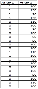
Now Sumproduct will multiply Array1 with Array 2 then will add up all individual values and result of the same will be 870 for salesman ABC, 840 for salesman PQR & 590 for salesman XYZ.

So in short advanced use of sumproduct is we can add condition to each range of sumproduct to get conditional result. i.e.

=SUMPRODUCT( (Range1=Condition1)*1, (Range2=Condition2)*1, (Range3=Condition3)*1,……, (Range n))

Where range n is values which we need as final result, here it is Sales Unit.

Also refer last sheet of attachment for more example of using SUMPRODUCT